Tutorial

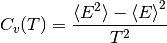
Calculating heat capacity,

#!/usr/bin/env python
import multiprocessing as mp
import os
import numpy as np
import pycabs


def runCABS(temperature):
	# global for simplify arguments 
	global name, sequence,secstr,template 
	
	# function for running CABS with different temperatures
	# it will compute in directory name+_+temperature
	here = os.getcwd() # since pycabs changing directories...
	a = pycabs.CABS(sequence,secstr,template,name+"_"+str(temperature))
	a.createLatticeReplicas(replicas=1)
	a.modeling(Ltemp=temperature,Htemp=temperature, phot=300,cycles=100,dynamics=True)
	#remember to come back to `here` directory
	os.chdir(here)


#init these variables _before_ running cabs
name = "fnord"
# we have some template, it has to be as list
template=["/home/user/pycabs/playground/2pcy.pdb"] 
# suppose we have porter prediction of sec. str.
sss =  pycabs.parsePorterOutput("/home/user/pycabs/proba/playground/porter.ss") 
sequence = sss[0]
secstr = sss[1]
# now we have all data required to run CABS

temp_from = 1.5
temp_to  = 3.0
temp_interval = 0.1
temperatures=np.arange(temp_from,temp_to,temp_interval) # ranges of temperature

# create thread pool  with two parallel threads
pool = mp.Pool(processes=2)
pool.map(runCABS,temperatures) # run cabs threads

# HERE IS THE END OF PART WHERE WE RUN CABS in parallel fashion. 

# Now you can do something with output data, we'll calculate heat capacity, Cv:
cv = np.empty(len(temperatures))
for i in range(len(temperatures)):
	t = temperatures[i]
	e_path = os.path.join(name+'_'+str(t),'ENERGY')
	energy = np.fromfile(e_path,sep='\n') # read ENERGY data into array `energy`
	avg_energy2 = np.average(energy*energy) # <E^2>
	avg_energy = np.average(energy)		    # <E>^2
	cv[i] = np.std(energy)*np.std(energy)/(t*t) # (<E^2> - <E>^2) / T^2
# now we have heat capacity in cv array	

# ... and display plot
from pylab import *
xlabel(r'temperature $T$')
ylabel(r'heat capacity $C_v = (\left<E^2\right> - \left<E\right>^2)/T^2$' )
xlim(temp_from,temp_to) # xrange
plot(temperatures,cv)
show()

#remember that you have name+_+temperature directories, delete it or sth

Download script: heat_capacity.py.

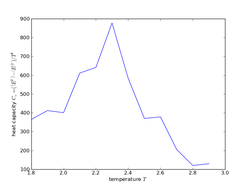
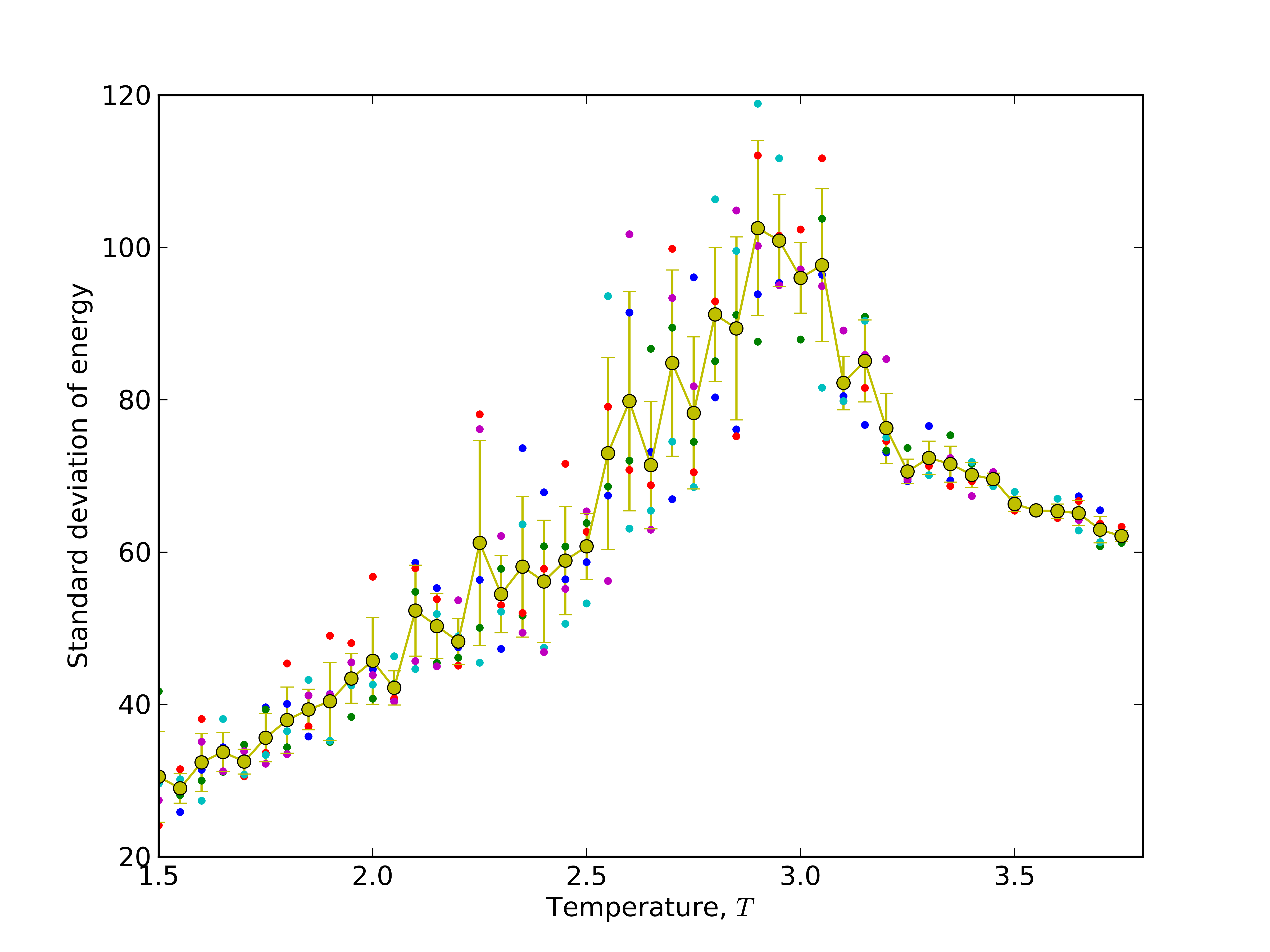
Study folding pathway: 1) create standard deviation and mean energy plots for Barnase

#!/usr/bin/env python
# 2013, Michal Jamroz, public domain. http://biocomp.chem.uw.edu.pl

import os, random, pylab, glob, pycabs, numpy as np, multiprocessing as mp
# first of all, download pyCABS and set self.FF = "" to the FF directory with cabs files
# to compile CABS, use: g77 -O2 -ffloat-store -static -o cabs CABS.f 
# to compile CABS_dynamics, use: g77 -O2 -ffloat-store -static -o cabs_dynamics CABS_dynamics.f 
# to compile lattice model builder, use g77 -O2 -ffloat-store -static build_cabs61.f
# in FF directory.

sequence, secstr = pycabs.parseDSSPOutput("/where/is/my/barnase/1bnr.dssp") # define file with secondary structure definition of define sequence and secondary structure in sequence,secstr variables respectively
name = "barnase" # name for the project. Script will create subdirectories with this name as suffix
template = ["/where/is/my/barnase/1bnr.pdb"] # set path to the start structure (here - native structure). If user want to start from random chain, set template=[]. Note that path is relative to simulation directory
independent_runs=5  # set number of independent simulations for each temperature
temp_from = 1.5     # define range of simulation temperatures, here is 1.0 - 2.8 with interval of 0.1
temp_to  = 3.8
temp_interval = 0.05
temperatures=np.arange(temp_from,temp_to,temp_interval)

def runCABS(temperature):
   global name, sequence,secstr,template,independent_runs
   here = os.getcwd()
   for i in range(independent_runs):
      temp = "%06.3f" %(temperature)
      dir_name= name+"_"+str(i)+"_T"+temp  # create unique name for simulation dir
      a = pycabs.CABS(sequence,secstr,template,dir_name) 
      a.rng_seed = random.randint(1,10000) # set random generator seed for each independent simulation
      a.createLatticeReplicas(replicas=1)  # create lattice model for CABS
      a.modeling(Ltemp=temperature,Htemp=temperature, phot=300,cycles=100,dynamics=True) # start modeling. phot is CABS microcycle, cycles variable is CABS macrocycle (how often write to the trajectory file)
      os.chdir(here)

pool = mp.Pool()  # it use all available CPUs on workstation. If user want to use only - for example two - CPUs, set pool = mp.Pool(2)
pool.map(runCABS,temperatures) # run simulations in parallel way, each simulation on each available CPU

# postprocessing (comment out two lines above to avoid starting over simulations. If you want to only plot with other labels, etc. )

cv = np.empty([independent_runs,len(temperatures)])
avgene = np.empty([independent_runs,len(temperatures)])
for j in range(independent_runs):
   for i in range(len(temperatures)):
      t = temperatures[i]
      temp = "%06.3f" %(t)
      e_path = os.path.join(name+'_'+str(j)+'_T'+temp,'ENERGY') # path constructed in the same way like dir_name in runCABS definition above
      energy = np.fromfile(e_path,sep='\n')[1000:] # read CABS energies for each trajectory model (second half)
      cv[j][i] = np.std(energy)  # calculate standard deviation (numpy std function) of energy, for each independent simulation
      avgene[j][i] = np.mean(energy) # calculate mean (numpy mean function) of energy


mean_sigma = np.mean(cv,axis=0)    # average over independent simulations
stddev_sigma = np.std(cv,axis=0)
mean_ene = np.mean(avgene,axis=0)  # calculate of standard deviations and mean values over independent simulations
stddev_ene = np.std(avgene,axis=0)

# plotting data with pylab python module. Read matplotlib manual (http://matplotlib.org/) for explanation of below code
pylab.ylabel(r'Standard deviation of energy' )
pylab.xlabel(r'Temperature, $T$')
pylab.xlim(temp_from,temp_to)
for i in range(independent_runs):
    pylab.plot(temperatures, cv[i], '.')
pylab.errorbar(temperatures,mean_sigma,yerr=stddev_sigma,fmt='o-')
pylab.savefig("stdE_barnase.png",dpi=600)
pylab.close()

pylab.ylabel(r'Mean energy' )
pylab.xlabel(r'Temperature, $T$')
pylab.xlim(temp_from,temp_to)
for i in range(independent_runs):
    pylab.plot(temperatures, avgene[i], '.')
pylab.errorbar(temperatures,mean_ene,yerr=stddev_ene,fmt='o-')
pylab.savefig("meanE_barnase.png",dpi=600)
pylab.close()


# as a results user will get a lot of barnase* subdirectories, stdE_barnase.png and meanE_barnase.png files.
# EOF

Download script: folding_pathway.py. Download necessary files: 1bnr.pdb, 1bnr.dssp

Results:

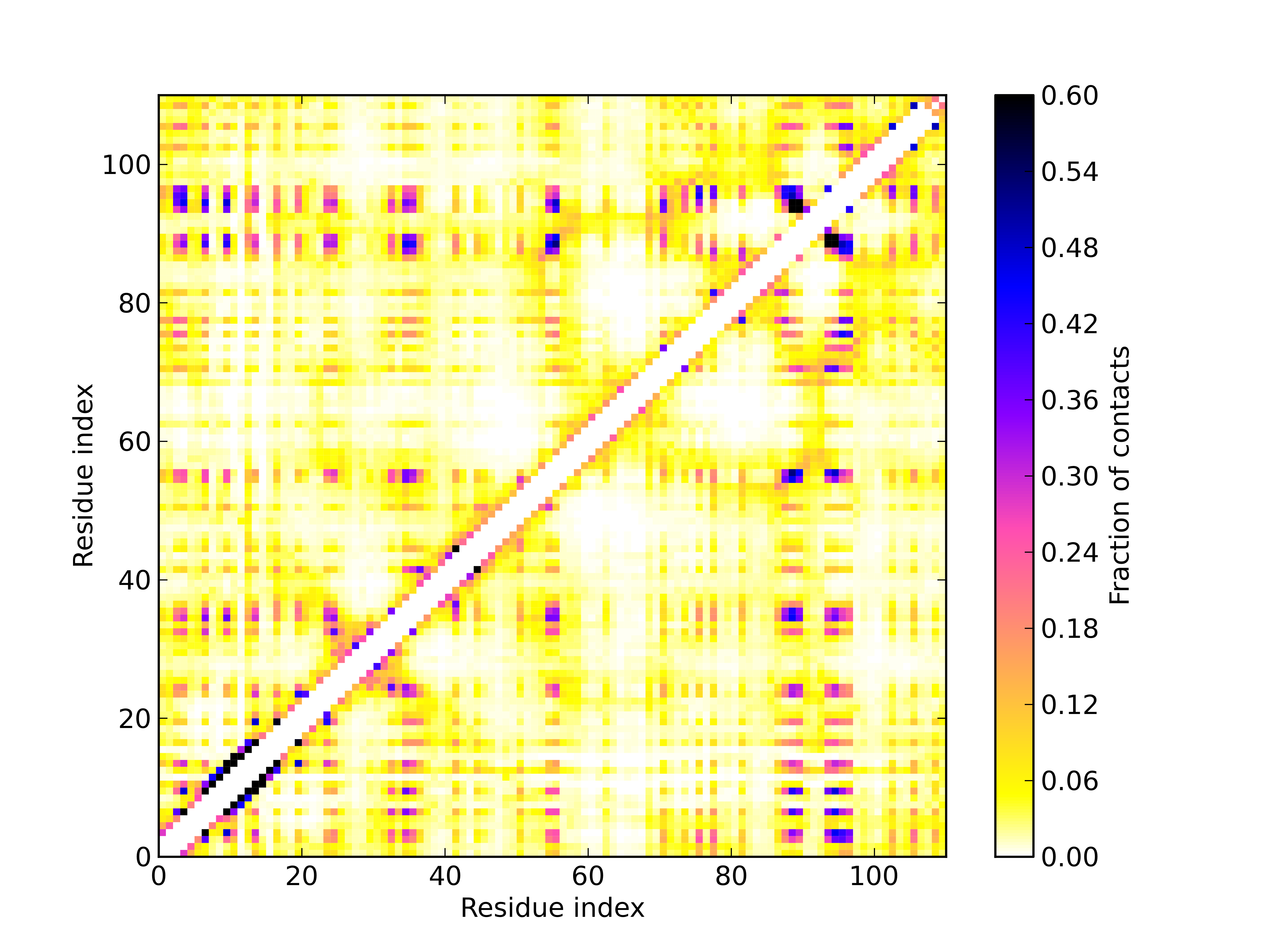
Study folding pathway: 2) calculate average contact map over trajectory of sidegroups in temperature 2.9

#!/usr/bin/env python
# 2013, Michal Jamroz, public domain. http://biocomp.chem.uw.edu.pl
import pycabs,os,numpy as np

name = "barnase" # set project name same like in folding_pathway.py script
max_sd_temperature=2.9 # read from the plot temperature for which maximum deviation of energy is observed
independent_runs=5     # set the same value like in folding_pathway.py script

# read trajectory of sidegroups (TRASG) from all independent simulations to the trajectory variable
trajectory = []
for j in range(independent_runs):
	temp = "%06.3f" %(max_sd_temperature)
	e_path = os.path.join(name+'_'+str(j)+'_T'+temp,'TRASG')
	trajectory += pycabs.loadSGCoordinates(e_path)[1000:] # second half of sidechains trajectory

contact = pycabs.contact_map(trajectory,7.0) # calculate averaged contact map over trajectories. Cutoff set to 7.0A.

# plot contact map with pylab. Read matplotlib manual (http://matplotlib.org/) for explanation of the code below
from pylab import xlabel,ylabel,pcolor,colorbar,savefig,xlim,ylim,cm
from numpy import indices
l=len(trajectory[0])
rows, cols = indices((l,l))
xlabel("Residue index")
xlim(0, len(contact))
ylim(0, len(contact))
ylabel("Residue index")
pcolor(contact, cmap=cm.gnuplot2_r,vmax=0.6) # vmax is range of colorbar. Here is set to 0.8, which gave white color for all values greater than 0.8
cb = colorbar()
cb.set_label("Fraction of contacts")
savefig("heatmap"+str(max_sd_temperature)+".png",dpi=600)

# optionally, write contact map values into the text file formatted for GNUplot
fw = open("contact_map.dat","w")
for i in range(len(contact)):
   for j in range(len(contact)):
      fw.write("%5d %5d %7.5f\n" %(i+1,j+1,contact[i][j]))
   fw.write("\n")
fw.close()

# example GNUplot script for plotting contact map of contact_map.dat file:
'''
set terminal unknown
plot 'contact_map.dat' using 1:2:3
set xrange[GPVAL_DATA_X_MIN:GPVAL_DATA_X_MAX]
set yrange[GPVAL_DATA_Y_MIN:GPVAL_DATA_Y_MAX]


set terminal postscript eps enhanced color "Helvetica" 14
set output 'contact_map.eps'
set size ratio 1
unset key
set xlabel 'Residue index'
set ylabel 'Residue index'
set cbrange[:0.8]
set palette negative
plot 'contact_map.dat' with image
'''

# write it to the file.gp and run: gnuplot file.gp to get postscript file with heat map plot

Download script: contact_map.py.

Results:

Optionally, GNUplot script for plotting contact_map.dat file generated by contact_map.py script:

set terminal unknown
plot 'contact_map.dat' using 1:2:3
set xrange[GPVAL_DATA_X_MIN:GPVAL_DATA_X_MAX]
set yrange[GPVAL_DATA_Y_MIN:GPVAL_DATA_Y_MAX]


set terminal postscript eps enhanced color "Helvetica" 14
set output 'contact_map.eps'
set size ratio 1
unset key
set xlabel 'Residue index'
set ylabel 'Residue index'
set cbrange[:0.8]
set palette negative
plot 'contact_map.dat' with image

Download script: gnuplot_script.gp.

Monitoring of CABS energy during simulation

#!/usr/bin/env python
from pylab import *
from sys import argv
import os
import time
import numpy as np
import pycabs

class Energy(pycabs.Calculate):
    def calculate(self,data):
        for i in data:
            self.out.append(float(i)) # ENERGY file contains one value in a row
            
out = []						
calc = Energy(out) # out is dynamically updated 
m=pycabs.Monitor(os.path.join(argv[1],"ENERGY"),calc)
m.daemon = True
m.start()



ion()
y = zeros(1)
x = zeros(1)
line, = plot(x,y)
xlabel('CABS time step')
ylabel('CABS energy')

while 1:
    time.sleep(1)
    y = np.asarray(out)
    x = xrange(0,len(out))
    axis([0, amax(x)+1, amin(y)-5, amax(y)+5 ])
    line.set_ydata(y)  # update the data
    line.set_xdata(x)
    draw()

Download script: monitoring_energy.py.

Monitoring of end-to-end distance of chain during simulation

#!/usr/bin/env python
from pylab import *
from sys import argv
import time
import os
import numpy as np
import pycabs

class E2E(pycabs.Calculate):
    def calculate(self,data):
        models = self.processTrajectory(data)
        for m in models:
            first = m[0:3]
            last = m[-3:]

            x = first[0]-last[0]
            y = first[1]-last[1]
            z = first[2]-last[2]
            self.out.append(x*x+y*y+z*z)            
            
out = []						
calc = E2E(out) # out is dynamically updated 
m=pycabs.Monitor(os.path.join(argv[1],"TRAF"),calc)
m.daemon = True
m.start()


ion()
y = zeros(1)
x = zeros(1)
line, = plot(x,y)
xlabel('CABS time step')
ylabel('square of end to end distance')

while 1:
    time.sleep(1)
    y = np.asarray(out)
    x = xrange(0,len(out))
    axis([0, amax(x)+1, amin(y)-5, amax(y)+5 ])
    line.set_ydata(y)  # update the data
    line.set_xdata(x)
    draw()

Download script: monitoring_e2e_distance.py.

De-novo modeling of 2PCY structure

#!/usr/bin/env python
import pycabs
from Pycluster import *
from numpy import array,zeros

data =  pycabs.parsePorterOutput("/home/user/pycabs/proba/playground/porter.ss") # read PORTER (or PsiPred) secondary structure prediction
working_dir = "de_novo" # name of project 
templates = [] # deNOVO
a = pycabs.CABS(data[0],data[1],templates,working_dir) # initialize CABS, create required files
# DENOVO a.generateConstraints() 
a.createLatticeReplicas() # create start models from templates
a.modeling(Htemp=3.0,cycles=20,phot=100) # start modeling with default INP values and create TRAF.pdb when done
tr = a.getTraCoordinates() # load TRAF into memory and calculate RMSD all-vs-all : 


#calculating RMSD 2D array for clustering
distances = zeros((len(tr),len(tr)))
for i in range(len(tr)):
	for j in range(i,len(tr)):
		rms = pycabs.rmsd(tr[i],tr[j])
		distances[i][j] = distances[j][i] = rms
		
#save RMSD array as heat map
pycabs.heat_map(distances,"Protein model","Protein model","RMSD")		


# clustering by K-medoids method (with 5 clusters)
clusterid,error,nfound = kmedoids(distances,nclusters=5,npass=15,initialid=None)
print clusterid,error
clusterid,error,nfound = kcluster(distances,nclusters=5,npass=15)

# save cluster medoids to file
pycabs.saveMedoids(clusterid,a)
print clusterid,error

Download script: de_novo.py.