Based on the example, see below how to
- 1. How to submit the job and interpret the status of processing
- 2. How to access and interpret the results data
- 2.1. Models tab
- 2.1.1. Multimodel subtab
- 2.1.2. Model 1, Model 2, …, Model X subtabs
- 2.2. Details tab
- 2.2.1. "Clustering data" subtab
- 2.2.2. "Cα RMSD and GDT_TS to the input structure" subtab
- 2.2.3. "Cα RMSD between predicted models" subtab
- 2.2.4. "Cα GDT_TS between predicted models" subtab
- 2.3. Superimposition by the Theseus application
- 3. Filling missing residues in PDB files
- 4. References
1. How to submit the job and interpret the status of processing
In order to submit the job you need to provide:
- the project name
- and the input structure in the form of: PDB structure code or protein structure file (in PDB format)
Mark the option “Do not show my job on the queue page” if you don’t want the job to be visible to anyone else on the queue page (QUEUE). The example of submitting the job named “example_1SUR” by providing the PDB code: “1SUR” is displayed below.

After clicking the Submit button, the following info will appear, which contain the unique link to your job:

If you have chosen “Do not show my job on the queue page” it is important to save the link to your job, otherwise your job will be accessible from the queue page: ( QUEUE).
Under the unique link to your job you’ll find the job status updates and finally the job results.
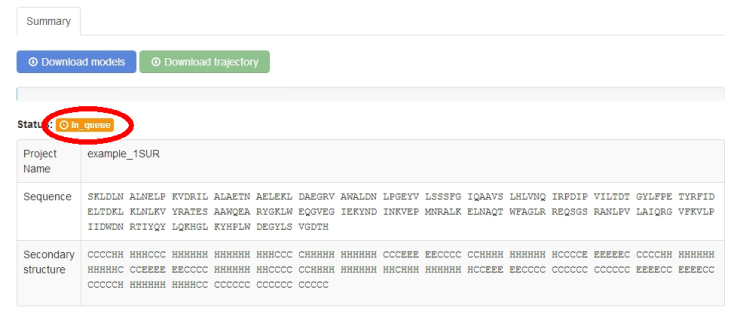
The job status information will start from the “in queue status”:

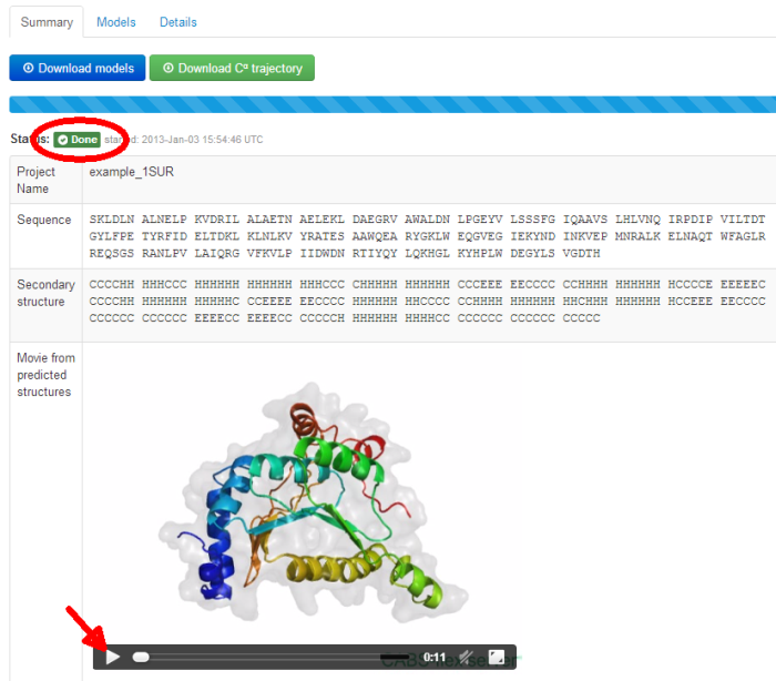
Additionally, a movie is automatically generated by creating frames from pictures of the predicted models in different rotation states. The movie can be viewed on-line (click play button) or downloaded (right-click on the movie screen and the option: “download the movie” should appear - the movie file will be in OGV or MP4 format, depending on a web browser).
2. How to access and interpret the results data
2.1. Models tab
Under the job link, the results are accessible from the Models menu tab (marked below in a red circle). Under the Models tab, results are divided into several sub-tabs (marked below in green circles):
- Multimodel
- Model 1, Model 2, Model 3, and subsequent ones (the number of the Models depend on the clustering results)
To see description of the displayed pictures, or the data to download (accessible under the blue buttons), drag the cursor over a picture, or a button.
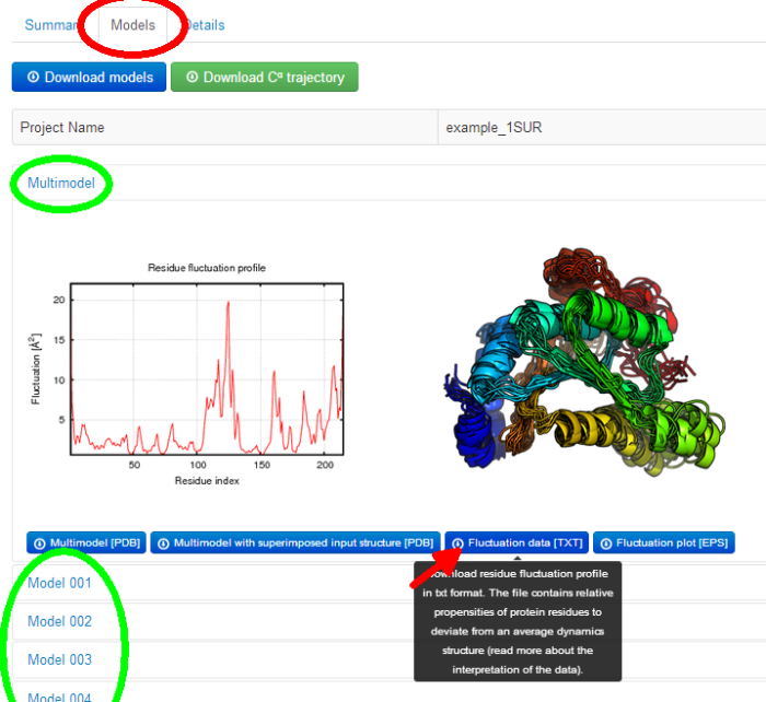
2.1.1. Multimodel subtab
The Multimodel subtab presents the following data:
- residue fluctuation profile in png, txt and eps format
- coordinates of the predicted models superimposed on each other (Model 1 and subsequent ones) in multi-model pdb file.
- coordinates of superimposed protein structures: the input (Model 1) and the predicted models (Model 2 and subsequent ones) in multi-model pdb file.
The superimposition is done by the Theseus application.
- the models picture presenting predicted models (in rainbow colors) superimposed on each other.
The picture is shown to provide at a glance visual information about the structural ensemble of predicted models. Note that, the models are displayed in a random orientation. In order to create your own customized molecular visualization picture, click the button below: "Multimodel [PDB]" and visualize the downloaded file with a molecular visualization software of your choice. See also Gallery of protein structure fluctuations resulted from the CABS-flex server.
The fluctuation of residue i was defined as in the [ ref 1]:

where j - trajectory frame, i - residue index, c - position of the Cα atom in the average structure, and N - number of trajectory models.
Residue fluctuation profile shows relative propensities of protein residues to deviate from an average dynamics (trajectory) structure. The CABS-flex employs simulation procedure from the work of [ ref 1], where it was demonstrated, that the average Spearman’s correlation coefficient for the fluctuations along protein chains between CABS and the atomic MD (all-atom, explicit water, for all protein metafolds using the four most popular force-fields) is average on the level of 0.7 (which has been confirmed in further test studies). Importantly, this level of correspondence is similar to that of between different MD force-fields.
The residue fluctuation values are also included into the final PDB output models (the temperature factor column, 61 – 66 columns in the PDB file, is replaced with the fluctuation values that can be visualized as colors using standard molecular visualization software).
2.1.2. Model 1, Model 2, …, Model X subtabs
The Model 1, Model 2 and each subsequent Model subtabs presents the following data:
- residue RMSD values (distances in Angstroms between residues of superimposed: the input structure and the predicted model) in png, txt and eps format
The superimposition is done by the Theseus application. The txt file contains an extra superimposition data provided by the Theseus. - coordinates of the predicted protein model in pdb format,
- coordinates of superimposed protein structures: the input (Model 1) and the predicted model (Model 2) in two-model pdb file,
- the models picture presenting the input structure (in red) and the predicted model (in rainbow colors) superimposed on each other.
The picture is shown to provide at a glance visual information about the similarity of the predicted model to the input structure. Note that, the structures are displayed in a random orientation. In order to create your own customized molecular visualization picture, click the button below: "Download model with superimposed input structure"). See also Gallery of protein structure fluctuations resulted from the CABS-flex server
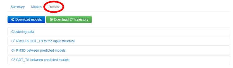
2.2. Details tab
Under the Details tab, results are divided into several sub-tabs:
- Clustering Data
- Cα RMSD and GDT_TS to the input structure
- Cα RMSD between predicted models
- Cα GDT_TS between predicted models
2.2.1. "Clustering data" subtab
Clustering of protein models is the task of separating a set of protein models (here a protein dynamics trajectory) into groups (called clusters). The clustering is done in such a way that models are more similar in the same group to each other (here in the sense of RMSD measure), than those in other groups (clusters). CABS-flex utilizes classical K-means clustering method.
After clustering is done, each cluster representative is chosen (always the model which average dissimilarity to all models in a cluster is minimal). Predicted protein models, presented in the Models tab, are each cluster representatives (the clusters and the corresponding models are marked by the same numbers, e.g. Model 1 represents Cluster 1).
The clusters are numbered/ranked according to cluster density values, from the most dense (numbered as a first) to the least dense one.
The subtab Clustering Data contains a table with the following clusters data:
- Cluster density values (cluster size divided by average cluster RMSD, rounded to one decimal place),
- Cluster size (numer of models grouped in a cluster).
Note that the number of models in the entire protein set (the dynamics trajectory of the input structure) is 2000 models, - Average cluster RMSD (average pairwise Cα RMSD value between models grouped in a cluster, rounded to one decimal place).
See the example table below:
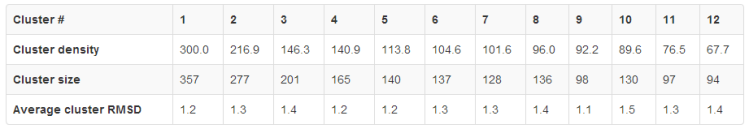
In the example above, the Cluster 1 contains 357 models (selected out of entire trajectory which contains 2000 models), whose average RMSD between all pairs of models in the Cluster is 1.2 Angstroms, and the Cluster density is 300 (note that the average cluster RMSD value given in the table is rounded to one decimal place, however in the calculation of the cluster density value the exact number is used).
Since the Cluster 1 is the most dense and most numerous, the Model 1 can be considered as the representative of the most dominant conformation in the entire fluctuation ensemble, followed by the Model 2 (representative of the second most dominant structure), and so on.
2.2.2. "Cα RMSD and GDT_TS to the input structure" subtab
The table contains RMSD and GDT_TS values (calculated on the Cα atoms) between the predicted models and the input structure. Note that GDT_TS metric is intended as a more accurate measurement than the more common RMSD.
Read more about the root-mean-square deviation (RMSD) measure
Read more about the global distance test (GDT, also written as GDT_TS to represent "total score") measure.
2.2.3. "Cα RMSD between predicted models" subtab
The table contains RMSD values (calculated on the Cα atoms) between the predicted models.
Read more about the root-mean-square deviation (RMSD) measure.
2.2.4. "Cα GDT_TS between predicted models" subtab
The table contains GDT_TS values (calculated on the Cα atoms) between the predicted models.
Read more about the global distance test (GDT, also written as GDT_TS to represent "total score") measure.
2.3. Superimposition by the Theseus application
The Theseus simultaneously superimposes multiple protein structures and finds the optimal solution to the superposition problem using the method of maximum likelihood. By downweighting variable regions of the superposition and by correcting for correlations among atoms, the maximum likelihood superpositioning method produces much more accurate results than conventional methods using least-squares criteria. Read more [ ref 2], Theseus website.
3. Filling missing residues in PDB files
CABS-flex requires input PDB files with continuous (without breaks) protein chain. PDB files with gaps in structure have to be first prepared by filling up the missing fragment. Below is the list of example software and on-line servers that enable filling in the gaps in incomplete 3D models:
- Modeller software
use Modeller to 'fill in' these missing residues by treating the original structure (without the missing residues) as a template, and building a comparative model using the full sequence
Availability: http://salilab.org/modeller/wiki/Missing%20residues - Modloop server
The server relies on the loop modeling routine in MODELLER that predicts the loop conformations by satisfaction of spatial restraints, without relying on a database of known protein structures
Availability: http://modbase.compbio.ucsf.edu/modloop/ - I-TASSER server
use with "Option I: Assign additional restraints and templates to guide I-TASSER modeling." You can use a PDB file with a missing fragment as a template and provide a missing fragment sequence in an alignment file
Availability: http://zhanglab.ccmb.med.umich.edu/I-TASSER/ - FALC-loop server
Users can submit a protein structure with one or more missing parts (called loops) through the Submit page and view and download the constructed loop models on the Queue page.
Availability: http://falc-loop.seoklab.org/ - FREAD server
FREAD is a database search loop modelling algorithm. Its primary use is to fill in the gaps in incomplete 3D models of protein structures
Availability: http://opig.stats.ox.ac.uk/webapps/fread - Commercial software
One can use also commercially available programs for loop sampling like Prime, ICM, and Sybyl (see comparison of these programs): http://www.ncbi.nlm.nih.gov/pmc/articles/PMC2206982/
4. References
- Jamroz M., Orozco M., Kolinski A., Kmiecik S. 2013, Consistent View of Protein Fluctuations from All-Atom Molecular Dynamics and Coarse-Grained Dynamics with Knowledge-Based Force-Field, J. Chem. Theory Comput., 9 (1), 119–125 doi: 10.1021/ct300854w
- Theobald, D. L., Wuttke D. S. (2006). THESEUS: Maximum Likelihood Superpositioning and Analysis of Macromolecular Structures. Bioinformatics 22 (17): 2171–2. doi:10.1093/bioinformatics/btl332.
© Laboratory of Theory of Biopolymers, Faculty of Chemistry, University of Warsaw 2013